2022 / Previous Year Question PYQ and answer / BBA / Microeconomics / AKU Bihar

1.Write True or False of any six of the following:

1. A consumer who is rational equates the marginal utility of all goods consumed.
2. Utility theory assumes that market ‘ baskets on higher indifference curves have higher utilities.
3. A consumer’s demand curve for a commodity generally will shift if the prices of other commodities change.
4. If a good is price elastic, a decrease in its price will result in a decrease in the amount of money spent on it.
5. Plant and equipment of a firm are fixed in the short run
6. Empirical studies often indicate the short-run average coat curve is S-shaped
7. If a firm’s price is fixed, then increase in output will have little effect on the firm’s profit
8. In the short run, equilibrium price under perfect competition may be
   above or below average total cost.
9. For a monopolist, marginal revenue is less than price.
10. Monopolistic competition is likely to result in more brands than perfect competition.

Answer:

(a) True
A rational consumer aims to maximize their total satisfaction (utility) with a limited budget. They achieve this by consuming goods up to the point where the marginal utility (MU) of the last unit consumed from each good is equal. This ensures they get the most “bang for their buck” from each purchase.

(b) True
Utility theory builds on the concept of indifference curves. These curves represent combinations of goods that provide the same level of satisfaction (utility) to a consumer. Higher indifference curves represent greater total utility.

(c) True
Changes in the price of other goods (called “substitute” or “complement” goods) can affect the demand for a particular commodity. For example, if the price of butter increases, a consumer might switch to margarine (substitute), potentially increasing the demand for margarine and decreasing the demand for butter.

(d) False
Price elasticity refers to the responsiveness of quantity demanded to a price change. If a good is price elastic (elastic demand), a decrease in price will lead to a greater than proportional increase in the quantity demanded, resulting in more money spent on the good (quantity effect outweighs price effect).

(e) True
In the short run, a firm’s plant and equipment capacity are considered fixed. They cannot be easily adjusted to accommodate significant changes in production levels.

(f) True
Empirical studies often show an S-shaped short-run average total cost (ATC) curve. This reflects economies of scale at lower production levels (decreasing ATC), followed by diseconomies of scale at higher levels (increasing ATC) due to inefficiencies or resource constraints.

(g) False
Even with a fixed price, increasing output can lead to higher profits as long as the marginal cost (MC) is less than the price. Each additional unit sold contributes to profit as long as the cost of producing it is less than the revenue it generates.

(h) True
In perfect competition, firms are price takers, meaning they accept the market price. In the short run, the equilibrium price may be above or below the average total cost due to factors like industry entry/exit or market disequilibrium.

(i) True
Monopolists have some control over price, but increased output lowers the price they can charge for each unit sold (due to the law of demand). This creates a gap between price (P) and marginal revenue (MR), where MR is less than P.

(j) True

Monopolistic competition leads to product differentiation and brand proliferation. Firms compete by creating unique product features, marketing strategies, and branding, resulting in a wider variety of brands compared to perfect competition, where firms offer identical products.

2. Short  Answer any three of the following :

Q2 A. What are different determinants of demand?

Answer

(a) Determinants of Demand: The main determinants of demand are:

1. Price of the Good: Generally, there is an inverse relationship between the price of a good and the quantity demanded.
2. Income of Consumers: Higher income typically increases demand for normal goods and decreases demand for inferior goods.
3. Prices of Related Goods:
   • Substitutes: An increase in the price of a substitute can increase demand for the good.
   • Complements: An increase in the price of a complement can decrease demand for the good.
4. Consumer Preferences: Changes in tastes and preferences can increase or decrease demand.
5. Expectations: If consumers expect prices to rise in the future, current demand may increase, and vice versa.
6. Number of Buyers: More buyers in the market increase the overall demand.
7. Seasonality: Certain times of the year can affect demand for specific products (e.g., holidays, weather changes).

Q2. B. Define marginal utility.

Answer

(b) Marginal Utility: Marginal utility is the additional satisfaction or benefit (utility) that a consumer derives from consuming an additional unit of a good or service. Mathematically, it is the change in total utility divided by the change in the quantity consumed: 𝑀𝑈=Δ𝑇𝑈/Δ𝑄

Q2 C . Define fixed cost and variable cost.

Answer:

(c) Fixed Cost and Variable Cost:

• Fixed Cost (FC): Costs that do not change with the level of output. They are incurred even if the firm produces nothing. Examples include rent, salaries of permanent staff, and insurance.
• Variable Cost (VC): Costs that vary directly with the level of output. As production increases, variable costs increase. Examples include raw materials, direct labor, and utilities.

Q2 D Explain kinked demand curve.

(d) Kinked Demand Curve: The kinked demand curve theory is used to explain price rigidity in oligopolistic markets. The curve has a distinct kink at the current price level:

• Above the Kink: The demand curve is relatively elastic because if a firm raises its price, other firms won’t follow, leading to a significant loss in market share.
• Below the Kink: The demand curve is relatively inelastic because if a firm lowers its price, other firms will also lower their prices, leading to only a small gain in market share. This results in a discontinuity in the marginal revenue curve, leading to price stability despite changes in marginal costs.

Q2. E. What is monopolistic competition?

(e) Monopolistic Competition: Monopolistic competition is a market structure characterized by:

• Many Firms: Numerous firms compete in the market.
• Product Differentiation: Each firm offers a product that is slightly different from the others, which gives them some degree of market power.
• Free Entry and Exit: Firms can freely enter or exit the market, which ensures that in the long run, firms will earn zero economic profit.
• Independent Decision-Making: Each firm makes independent decisions about prices and output based on their product, costs, and market conditions. This market structure results in a variety of products available to consumers and encourages innovation and advertising as firms strive to differentiate their products.

Long Answer question

Q. Differentiate between price elasticity of demand and income elasticity of demand. Explain different methods for measurement of price elasticity of demand.

Answer:

1. Differentiating between Price Elasticity of Demand and Income Elasticity of Demand:

Price Elasticity of Demand (PED):

• Definition: Price elasticity of demand measures how much the quantity demanded of a good responds to a change in its price.
• Formula: PED=% change in quantity demanded / % change in price
• Interpretation:
  • Elastic Demand (PED > 1): Quantity demanded changes by a greater percentage than the price change.
  • Inelastic Demand (PED < 1): Quantity demanded changes by a smaller percentage than the price change.
  • Unit Elastic Demand (PED = 1): Quantity demanded changes by the same percentage as the price change.
  • Perfectly Elastic (PED = ∞): Quantity demanded changes infinitely with any small change in price.
  • Perfectly Inelastic (PED = 0): Quantity demanded does not change with a change in price.

Income Elasticity of Demand (YED):

• Definition: Income elasticity of demand measures how much the quantity demanded of a good responds to a change in consumers’ income.
• Formula:
• YED=% change in quantity demanded / % change in income
• Interpretation:
  • Positive YED (> 0): The good is a normal good. Higher income increases demand.
  • Negative YED (< 0): The good is an inferior good. Higher income decreases demand.
  • High YED (> 1): The good is a luxury good. Demand increases more than proportionally as income rises.
  • Low YED (0 < YED < 1): The good is a necessity. Demand increases less than proportionally as income rises.

2. Different Methods for Measurement of Price Elasticity of Demand:

Percentage Method:

• Formula: PED=% change in quantity demanded / % change in price
• Application: This method uses the initial and final quantities and prices to calculate the percentage changes.

Total Revenue (Expenditure) Method:

• Concept: Observes changes in total revenue (price multiplied by quantity) as price changes.
  • Elastic Demand: If total revenue increases when price decreases (or decreases when price increases).
  • Inelastic Demand: If total revenue decreases when price decreases (or increases when price increases).
  • Unit Elastic Demand: Total revenue remains unchanged when price changes.

Arc Elasticity (Midpoint) Method:

• Formula: PED=(𝑄2−𝑄1) / (𝑄1+𝑄2)/2) /    (𝑃2−𝑃1)/(𝑃1+𝑃2)/2)​
• Application: This method calculates elasticity over a range of prices and quantities, using the average of the initial and final values to provide a more accurate measure.

Point Elasticity Method:

• Formula: PED=∂𝑄/∂𝑃 × 𝑃/ 𝑄
• Application: This method uses calculus to find the elasticity at a specific point on the demand curve, particularly useful for small changes in price.

Graphical Method:

• Concept: Measures elasticity based on the slope of the demand curve.
  • Elastic Demand: Flatter demand curve.
  • Inelastic Demand: Steeper demand curve.
  • Unit Elastic Demand: A demand curve that has a constant elasticity along its length.

These methods provide various ways to quantify how sensitive the quantity demanded is to changes in price, helping businesses and economists make informed decisions.

Q . “The indifference curve analysis has been a major advance in the field of consumer’s  demand ’ Critically examine this statement

Answer:

Critical Examination of Indifference Curve Analysis

The indifference curve analysis has indeed been a significant advancement in the field of consumer demand theory, providing a more nuanced understanding of consumer preferences and the choices they make. Let’s explore this statement critically and illustrate it with a graph.

Key Advancements of Indifference Curve Analysis:

1. Preference Representation:
   • Indifference curves represent combinations of goods that give the consumer the same level of satisfaction. This graphical representation helps in understanding consumer preferences without requiring numerical values for utility.
   • Each indifference curve represents a different level of utility, with curves further from the origin indicating higher utility levels.
2. Marginal Rate of Substitution (MRS):
   • The slope of an indifference curve at any point is the marginal rate of substitution (MRS), which shows the rate at which a consumer is willing to trade one good for another while remaining on the same indifference curve.
   • This concept illustrates the consumer’s willingness to substitute between goods, capturing the trade-offs they are willing to make.
3. Consumer Equilibrium:
   • By combining indifference curves with a budget constraint, the analysis determines the consumer’s equilibrium point where the highest attainable indifference curve is tangent to the budget line.
   • This tangency point reflects the optimal consumption bundle where the MRS equals the ratio of the prices of the two goods (MRS = 𝑃𝑥/𝑃𝑦Px​/Py​).

Graphical Illustration:

Below is a simplified graph illustrating these concepts:

• Indifference Curves (IC1, IC2, IC3): Curves representing different levels of utility. Higher curves (e.g., IC3) represent higher utility.
• Budget Line (BL): Represents all combinations of two goods (X and Y) that the consumer can afford given their income and prices of goods.
• Consumer Equilibrium (E): Point where the highest attainable indifference curve (IC2) is tangent to the budget line, indicating the optimal consumption bundle.

Critical Examination:

Strengths:

1. Flexibility in Preferences:
   • Indifference curves can accommodate any type of preferences, including those that are not easily quantifiable, thus offering a more flexible and realistic representation of consumer behavior.
2. Insight into Substitution Effects:
   • The MRS provides valuable insight into how consumers substitute between goods, enhancing the understanding of consumer choice dynamics.
3. Non-Monetary Utility:
   • Unlike utility functions that require numerical values, indifference curves work with ordinal utility, which only requires ranking preferences rather than quantifying them.

Limitations:

1. Complexity in Real-World Application:
   • While theoretically robust, the practical application of indifference curve analysis can be complex, as it requires detailed information about consumer preferences and budget constraints.
2. Assumption of Rationality:
   • Indifference curve analysis assumes that consumers are rational and always make choices to maximize their utility. Real-world behavior often deviates from this assumption due to factors like bounded rationality and irrational preferences.
3. Static Analysis:
   • The analysis typically considers a static framework, ignoring the effects of changes over time, such as income changes, price fluctuations, and preference shifts.

Indifference curve analysis has significantly advanced the understanding of consumer demand by providing a flexible and detailed framework for analyzing consumer choices and preferences. Despite its complexity and some unrealistic assumptions, it remains a powerful tool in economics, enriching both theoretical insights and practical applications in consumer behavior analysis.

Q. Distinguish between laws of returns to variable proportions and laws of returns to scale. What factors cause increasing returns to scale?

Answer:

1. Laws of Returns to Variable Proportions (Short Run)

Definition:

• The laws of returns to variable proportions describe how output changes as the quantity of one input (typically labor) is varied while other inputs (capital, land) are held constant.
• This is a short-run concept where at least one factor of production is fixed.

Phases:

1. Increasing Returns to Variable Proportions:
   • Initially, as more units of the variable input are added to fixed inputs, output increases at an increasing rate due to better utilization of the fixed inputs.
2. Diminishing Returns to Variable Proportions:
   • Eventually, adding more units of the variable input leads to output increasing at a decreasing rate. This happens because the fixed inputs become overutilized, leading to less efficient production.
3. Negative Returns to Variable Proportions:
   • Finally, adding more units of the variable input can cause total output to decline as the inefficiencies from overcrowding and overuse of fixed inputs become significant.

2. Laws of Returns to Scale (Long Run)

Definition:

• The laws of returns to scale describe how output changes when all inputs (both labor and capital) are varied in the same proportion.
• This is a long-run concept where all factors of production are variable.

Phases:

1. Increasing Returns to Scale:
   • Output increases by a greater proportion than the increase in inputs. For example, doubling all inputs may more than double output.
2. Constant Returns to Scale:
   • Output increases in the same proportion as the increase in inputs. For example, doubling all inputs exactly doubles output.
3. Decreasing Returns to Scale:
   • Output increases by a smaller proportion than the increase in inputs. For example, doubling all inputs results in less than double the output.

Factors Causing Increasing Returns to Scale:

1. Specialization and Division of Labor:
   • As a firm scales up, workers can specialize in specific tasks, increasing productivity and efficiency.
2. Technical and Managerial Efficiency:
   • Larger firms can afford advanced technology and better management practices that smaller firms cannot, leading to more efficient production.
3. Economies of Scale:
   • Larger firms benefit from economies of scale, such as bulk purchasing of materials, more favorable financing rates, and spreading fixed costs over a larger output.
4. Learning and Experience:
   • As firms produce more, they learn and improve their production processes, leading to greater efficiency and lower costs over time.
5. Indivisibilities:
   • Some inputs cannot be scaled down for smaller levels of production, so increasing the scale of production can make better use of these indivisible resources.

 

Q. Why do monopoly firms adopt discriminatory pricing policy? Under what conditions is price discrimination desirable and profitable?

Answer:

Monopoly firms adopt discriminatory pricing policies to maximize their profits by capturing more consumer surplus and converting it into producer surplus. Price discrimination involves charging different prices to different consumers for the same good or service based on their willingness to pay, rather than charging a single, uniform price.

Reasons for Adopting Price Discrimination:

1. Profit Maximization:
   • By charging higher prices to consumers who are willing to pay more and lower prices to those who are more price-sensitive, a monopoly can increase its total revenue and profits compared to charging a single price.
2. Market Segmentation:
   • Price discrimination allows firms to segment the market based on differences in price elasticity of demand. Different segments can be charged differently to reflect their varying demand sensitivities.
3. Utilization of Market Power:
   • Monopolies can leverage their control over the market to implement price discrimination without facing significant competition that would otherwise erode their ability to charge different prices.

Conditions for Price Discrimination to be Desirable and Profitable:

1. Market Power:
   • The firm must have some control over the market price, typically because it is a monopoly or holds significant market power.
2. Ability to Segment Markets:
   • The firm must be able to segment the market into distinct groups based on their willingness to pay. This requires information about consumers’ preferences and the ability to prevent arbitrage (resale between consumers).
3. Different Elasticities of Demand:
   • The different consumer groups must have varying price elasticities of demand. Price-sensitive consumers should be charged lower prices, while less price-sensitive consumers can be charged higher prices.
4. Prevention of Arbitrage:
   • The firm must be able to prevent or limit resale between consumers paying different prices. If consumers who are charged lower prices can resell to those facing higher prices, the effectiveness of price discrimination is undermined.
5. Legal and Ethical Constraints:
   • Price discrimination must comply with legal and regulatory frameworks. Some forms of price discrimination may be illegal or deemed unethical, depending on the jurisdiction and context.

Types of Price Discrimination:

1. First-Degree (Perfect) Price Discrimination:
   • Charging each consumer the maximum price they are willing to pay. This captures all consumer surplus as profit but requires detailed knowledge of each consumer’s willingness to pay.
2. Second-Degree Price Discrimination:
   • Charging different prices based on the quantity consumed or the version of the product. Examples include bulk discounts and product versions with different features.
3. Third-Degree Price Discrimination:
   • Charging different prices to different consumer groups based on observable characteristics such as age, location, or time of purchase. Examples include student discounts, senior citizen discounts, and peak vs. off-peak pricing.

Examples:

1. Airlines:
   • Airlines often practice third-degree price discrimination by charging different prices based on booking time, class of service, and flexibility of the ticket.
2. Software Companies:
   • Software companies might use second-degree price discrimination by offering different versions of their products (e.g., basic, professional, enterprise) at different price points.

Thus monopoly firms adopt discriminatory pricing policies to maximize profits by extracting more consumer surplus. Price discrimination is desirable and profitable under conditions where the firm has market power, can segment the market, faces different demand elasticities, and can prevent arbitrage. Legal and ethical considerations also play a role in determining the appropriateness of such practices.

Q. Explain price and output determination under the condition of perfect competition in the short run and in the long run. Illustrate your answer graphically

Answer:

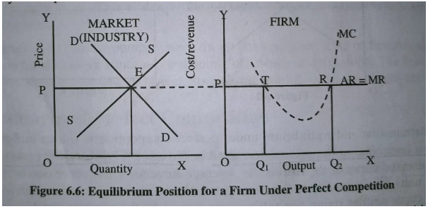
Conditions of Price and Output Determination Under Perfect Competition

Under perfect competition price of goods is determined by industry of forces of demand and supply. Equilibrium price is determined at a point where market demand is equal to market supply

A firm under the perfect condition is Price taker not price maker

›TWO Main Condition

›1.) A marginal revenue must be at least equal to the marginal cost, that is, MR=MC.

› If MR is higher than MC, there is always a reason for the company to increase production even more and profit after selling extra costs instead of reducing output, as the additional unit is more to the cost than revenue. Profits are maximum only at the point where MR=MC.

›2.) The MC Curve should cut the MR curve below.

Price and Output Determination Under Perfect Competition:

1) If AR > AC, the firm will receive super normal profits.

2) If AR is equal to AC, the company will earn normal profits (i.e., break-even)
3) If AR is less than AC the company will incur a loss.
4) If AR is less than AVC the company will cease production.(shutdown)

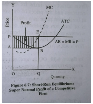
›1) Abnormal Profit/Supernormal Profit

›A business may make unusual profits at the equilibrium level of output when its average earnings exceed the cost of production by an average.

›In diagram 6.7, the firm’s equilibrium is at point E when the MC curve meets with the MR curve. When the firm is at OP prices, the company generates OQ output.

›The company’s average income (AR) equals EQ when it produces OQ output.

›Its average cost (AC) will be BQ because AR is higher than AC. Firms get abnormal profits. In the end, companies experience abnormal profits (EB) in unit output.

›It is the total profits (PABE), the per-unit profit divides by total output.

2) Normal profits or Break-Even

›If the company only covers its total costs, it makes normal profits.
Here AR = ATC

›Figure 6.9 illustrates how MR=MC at E.

›The final output of the equilibrium is called OQ. Since AR=ATC or OP=EQ, the company gets normal profits.

3.) If AR is less than AC (AR<AC) the company will incur a loss.

›In the event of an equilibrium output, firms can suffer losses. A seller might not recoup a portion of fixed costs in the short term. Despite these losses, the company may choose to produce to cover its average variable costs.

›In figure 6.8. The equilibrium value and, at this point, AR=EQ while AC=BQ as BQ is greater than EQ. The firm earns BE per loss unit, and the total loss is the amount of ABEP.

4) If AR is less than AVC the company will cease production.(shutdown)

Shut Down Point:

The firm will continue producing till the price covers the average variable cost. If the price covers some part of the o average fixed costs besides the variable cost, the producer will continue producing.

Thus the firm will continue producing so long as price exceeds the average variable cost.

but if price fall below the AVC  it will not continue to produce and firm has to shut down operation in short run

›The shutdown point can be shown with the help of a diagram: In the diagram, equilibrium is at E where MR = MC and MC cuts MR from below. The price is EQ and OQ is the output.

›This price covers the average variable cost and some portion of AFC i.e. NE but still per unit loss is AE but the firm will continue production as if it stops production loss per unit will form AN i.e. difference between AC & AVC     i.e, AFC (AQ – NQ = AN).

›If the market price falls to OP1 only AVC is covered i.e. E1Q1 = OP1, Now there will not be any use to continue production and so E1 will be shut down point.

ATC =AQ, revenue= EQ, AFC= AN, AVC= NQ revenue after price fall =SQ

Price and output Determination and Equilibrium of the Firm in the Long Run

›In the long run company earns only normal profit

›Why not super normal profit ? Because supernormal profit will attract many players to the market which will reduce the profit

›Why not minimum losses? Because no firms can survive on losses on long run.

›Free entry and exit play a crucial role in the long run. If any firm earns economic profits (price exceeds Average Total Cost (ATC)), new firms will enter the market, increasing supply and driving down the price.

›Conversely, if firms incur losses (price falls below ATC), some firms will exit the market, reducing supply and pushing the price up.

›This process continues until all firms reach long-run equilibrium, where price equals ATC (AR = AC = MC = MR) at the minimum point of the long-run average cost (LAC) curve. This is also known as the normal profit level, where firms earn neither profits nor losses but are able to cover all their costs.

›All firms are at break-even because of the loss of profits. It results from the long-term equilibrium between the industry and firm in a perfect market. Also, price and output determination under perfect competition, whereas all firms break even and make regular profits in the long term. Firms operate in a zero-loss-no-profit scenario where AR=AC is graphically plots in Figure 6.10.

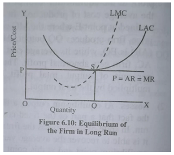
›In figure 6.10, in this output stage, the price and output determination under perfect competition is as the average revenue and average cost are the same as QS, while OQ represents the equilibrium value. Because of this, the firm will only earn regular profits. In this case, as the average cost is low, the average and marginal costs will remain the same, so the long-term equilibrium conditions for a business will be: MR=LMC=LAC= Price.