2019 previous year question PYQ with answer BBA AKU Bihar Microeconomics /

2019 / previous year question PYQ with answer / BBA / Microeconomics / AKU Bihar

1. Very Short Answer Type Questions

Answer any six of the following :             

(a)          Define demand.

(b)          Explain elasticity of demand.

(c)           What do you understand by supply?

(d)          Define utility.

(e)          The law of marginal utility theory is based on which measurement of utility?

(f)           What is the normal shape of an indifference curve?

(g)          Name the different costs relevant in short-run only.

(h)          Define production function.

(i)            In which type of competitive market advertisement is needed?

(j)             How firm and industry are related?

Answer

(a) Demand:

Definition:
Demand refers to the quantity of a good or service that consumers are willing and able to buy at various prices during a specific period, holding all other factors constant.

(b) Elasticity of Demand:

Explanation:
Elasticity of demand measures how sensitive the quantity demanded of a good or service is to a change in its price. It is calculated as the percentage change in quantity demanded divided by the percentage change in price.

Interpretation:

• Elastic Demand: When the percentage change in quantity demanded is greater than the percentage change in price (|E| > 1).
• Inelastic Demand: When the percentage change in quantity demanded is less than the percentage change in price (|E| < 1).
• Unitary Elastic Demand: When the percentage change in quantity demanded is equal to the percentage change in price (|E| = 1).

(c) Supply:

Definition:
Supply refers to the quantity of a good or service that producers are willing and able to offer for sale at various prices during a specific period, holding all other factors constant.

(d) Utility:

Definition:
Utility refers to the satisfaction or benefit that consumers derive from consuming a good or service. It is subjective and varies from person to person and across different circumstances.

(e) Law of Marginal Utility Theory:

Measurement of Utility:
The law of marginal utility theory is based on the ordinal measurement of utility. This means that utility is ranked or ordered according to preferences, rather than being measured in absolute or cardinal terms.

(f) Normal Shape of an Indifference Curve:

Shape:
The normal shape of an indifference curve is concave to the origin. This shape indicates that as a consumer moves along the curve, trading off one good for another, they are willing to give up less and less of one good to obtain additional units of the other good while remaining indifferent in terms of satisfaction.

(g) Different Costs Relevant in the Short Run Only:

Relevant Costs:
In the short run, the relevant costs include:

1. Variable Costs: Costs that vary with the level of production.
2. Total Fixed Costs: Costs that remain constant regardless of the level of production.
3. Average Variable Costs: Variable costs per unit of output.
4. Marginal Costs: The additional cost incurred by producing one more unit of output.

(h) Production Function:

Definition:
A production function represents the relationship between inputs (factors of production) and outputs (goods or services) produced by a firm. It shows the maximum quantity of output that can be produced from a given set of inputs.

(i) Competitive Market Requiring Advertisement:

Market Type:
In monopolistic competition, advertisement is often needed. In this market structure, firms produce similar but differentiated products, and they engage in non-price competition, such as advertising, to distinguish their products and attract customers.

Q2.  short Answer  type   Question

Answer any three of the following :

2 (a) What are the factors that determine demand for normal goods?

Answer:

(a) Factors that Determine Demand for Normal Goods

1. Income: For normal goods, as consumer income increases, the demand for these goods also increases. Conversely, a decrease in income leads to a decrease in demand.
2. Price of the Good: Generally, a decrease in the price of a normal good leads to an increase in quantity demanded, and an increase in price leads to a decrease in quantity demanded.
3. Prices of Related Goods: The demand for a normal good can be affected by the prices of complementary and substitute goods. If the price of a complementary good falls, demand for the normal good may increase. If the price of a substitute good falls, demand for the normal good may decrease.
4. Tastes and Preferences: Changes in consumer preferences and trends can increase or decrease demand for normal goods.
5. Expectations: If consumers expect prices to rise in the future, they may increase their current demand. Conversely, if they expect prices to fall, they may decrease their current demand.
6. Population: An increase in the population generally leads to an increase in demand for normal goods, assuming other factors remain constant.
7. Consumer Confidence: Higher consumer confidence in the economy can lead to increased spending on normal goods.

2 (b) Describe the concept of income elasticity of demand.

Answer:

(b) Income Elasticity of Demand

The income elasticity of demand measures the responsiveness of the quantity demanded of a good to a change in consumer income. It is calculated as:

𝐸𝐼=%Δ𝑄𝑑/ %Δ𝐼​​

where %Δ𝑄𝑑​ is the percentage change in quantity demanded and %Δ𝐼 is the percentage change in income.

• Positive Income Elasticity: Indicates that the good is a normal good. Higher income leads to higher demand.
• Negative Income Elasticity: Indicates that the good is an inferior good. Higher income leads to lower demand.
• High Income Elasticity: Goods with a high positive income elasticity are often luxury items.
• Low Income Elasticity: Goods with a low positive income elasticity are often necessities.

2(c) Explain the law of diminishing marginal utility theory.

Answer:

(c) Law of Diminishing Marginal Utility Theory

The law of diminishing marginal utility states that as a person consumes more units of a good or service, the additional satisfaction (utility) obtained from consuming each additional unit decreases.

For example, the first slice of pizza may provide a high level of satisfaction, but by the fourth or fifth slice, the additional satisfaction gained from consuming another slice will be less. This concept is crucial in understanding consumer choice and demand, as it implies that consumers will only continue to consume more of a good if its price decreases.

2(d) What is iso-cost? Explain.

Answer:

(d) Iso-cost

An iso-cost line represents all combinations of inputs (usually labor and capital) that a firm can purchase for a given total cost. The equation for an iso-cost line is:

𝐶=𝑤𝐿+𝑟𝐾

where 𝐶is the total cost, 𝑤w is the wage rate of labor, 𝐿 is the quantity of labor, 𝑟is the rental rate of capital, and 𝐾 is the quantity of capital.

The iso-cost line helps firms determine the most cost-effective combination of inputs. It is similar to a budget constraint in consumer theory.

2(e) Explain oligopoly market.

Answer:

(e) Oligopoly Market

An oligopoly is a market structure characterized by a small number of firms that dominate the market. Key features of an oligopoly include:

1. Few Sellers: Only a few firms control a large portion of the market.
2. Interdependence: Firms in an oligopoly are interdependent, meaning the actions of one firm affect the others. This often leads to strategic behavior and game theory analysis.
3. Barriers to Entry: High barriers to entry prevent new firms from entering the market easily. These barriers can be due to high startup costs, control over essential resources, or regulatory obstacles.
4. Price Rigidity: Prices in an oligopoly tend to be stable because firms are wary of starting price wars, which can be damaging to all competitors.
5. Non-Price Competition: Firms often compete using non-price strategies such as advertising, product differentiation, and customer service enhancements.
6. Collusion: There is a potential for firms to collude, either explicitly or tacitly, to set prices or output levels to maximize collective profits.

Oligopolistic markets include industries like automobile manufacturing, airlines, and telecommunications.

Long Answer Type Question

Q. Explain and distinguish a shift in the demand curve and a movement along a demand curve.

Answer:

Shift in the Demand Curve vs. Movement Along the Demand Curve

Movement Along the Demand Curve

A movement along the demand curve occurs when there is a change in the quantity demanded due to a change in the price of the good itself, with all other factors remaining constant. This movement can either be:

• Upward Movement (Contraction): When the price increases, the quantity demanded decreases, resulting in an upward movement along the demand curve.
• Downward Movement (Expansion): When the price decreases, the quantity demanded increases, resulting in a downward movement along the demand curve.

Graphical Representation:

In the graph below, the original demand curve is represented by 𝐷D.

• Point A to B shows a downward movement (price decrease from 𝑃1​ to 𝑃2​ and quantity increase from 𝑄1​ to 𝑄2​).
• Point B to A shows an upward movement (price increase from 𝑃2P2​ to 𝑃1P1​ and quantity decrease from 𝑄2​ to 𝑄1​).

Shift in the Demand Curve

A shift in the demand curve occurs when there is a change in any non-price determinant of demand, such as consumer income, preferences, prices of related goods, expectations, or number of buyers. This shift can either be:

• Rightward Shift (Increase in Demand): Indicates that at every price level, the quantity demanded is higher. This could be due to factors like higher income, increased preference for the good, or a rise in the price of a substitute good.
• Leftward Shift (Decrease in Demand): Indicates that at every price level, the quantity demanded is lower. This could be due to factors like lower income, decreased preference for the good, or a rise in the price of a complementary good.

Graphical Representation:

In the graph below, the original demand curve is 𝐷1​.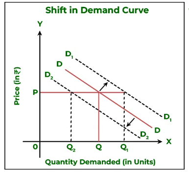

• 𝐷1​ to 𝐷2​ shows a rightward shift (increase in demand).
• 𝐷1 to 𝐷3​ shows a leftward shift (decrease in demand).

Key Differences:

• Cause:
  • Movement along the curve is caused by a change in the price of the good.
  • Shift in the curve is caused by changes in non-price factors (income, preferences, etc.).
• Result:
  • Movement along the curve results in a different quantity demanded at the same price.
  • Shift in the curve results in a different demand curve, indicating a different quantity demanded at every price.

• A movement along the demand curve represents a change in the quantity demanded due to a price change, moving from one point to another on the same demand curve.
• A shift in the demand curve represents a change in demand due to non-price factors, resulting in a completely new demand curve either to the right (increase) or to the left (decrease).

Q. Discuss price elasticity of demand and  compare with income elasticity of demand.

Price Elasticity of Demand (PED)

Definition: Price Elasticity of Demand (PED) measures how much the quantity demanded of a good responds to a change in its price. It is a key concept in understanding consumer behavior and market dynamics. The formula for calculating PED is:

𝑃𝐸𝐷=%Δ𝑄𝑑 / %Δ𝑃    ​​

where %Δ𝑄𝑑​ is the percentage change in quantity demanded and %Δ𝑃 is the percentage change in price.

Types of Price Elasticity:

1. Elastic Demand (PED > 1): A small change in price leads to a large change in quantity demanded. Examples include luxury goods and goods with many substitutes.
2. Inelastic Demand (PED < 1): A change in price leads to a small change in quantity demanded. Examples include necessities like food and medicine.
3. Unitary Elastic Demand (PED = 1): A change in price leads to a proportional change in quantity demanded.
4. Perfectly Elastic Demand (PED = ∞): Quantity demanded changes infinitely with a tiny change in price. This is theoretical and rarely seen in real life.
5. Perfectly Inelastic Demand (PED = 0): Quantity demanded remains unchanged regardless of price changes. Examples include life-saving drugs.

Factors Influencing PED:

• Availability of Substitutes: Goods with many substitutes tend to have higher elasticity.
• Necessity vs. Luxury: Necessities tend to have inelastic demand, while luxuries have elastic demand.
• Proportion of Income: Goods that take up a large portion of income tend to have higher elasticity.
• Time Horizon: Demand is generally more elastic over the long term as consumers can adjust their behavior.

Implications for Businesses and Policymakers:

• Pricing Strategies: Firms can use knowledge of PED to set prices optimally. For elastic goods, lowering prices can increase total revenue.
• Taxation Policies: Governments consider PED when imposing taxes. Taxes on inelastic goods generate more revenue with less impact on quantity demanded.
• Subsidies: Understanding PED helps in deciding which goods to subsidize to achieve desired economic outcomes.

Income Elasticity of Demand (YED)

Definition: Income Elasticity of Demand (YED) measures how much the quantity demanded of a good responds to a change in consumers’ income. The formula for calculating YED is:

𝑌𝐸𝐷=%Δ𝑄𝑑 / %/Δ𝐼​​

where %Δ𝑄𝑑 is the percentage change in quantity demanded and %Δ𝐼 is the percentage change in income.

Types of Income Elasticity:

1. Positive Income Elasticity (YED > 0): Demand for the good increases as income increases. Normal goods fall into this category.
   • Necessities (0 < YED < 1): Demand increases with income but at a decreasing rate. Examples include basic food items and clothing.
   • Luxuries (YED > 1): Demand increases with income at an increasing rate. Examples include high-end electronics and luxury cars.
2. Negative Income Elasticity (YED < 0): Demand for the good decreases as income increases. Inferior goods fall into this category. Examples include generic brands or budget products.

Factors Influencing YED:

• Nature of the Good: Whether the good is a necessity, luxury, or inferior good.
• Consumer Preferences: Changes in preferences and societal norms can affect how demand responds to income changes.
• Income Distribution: How income changes are distributed across different consumer groups can impact overall demand for various goods.

Implications for Businesses and Policymakers:

• Product Planning: Firms can use YED to predict changes in demand based on economic conditions. Luxury goods manufacturers might target markets with rising incomes.
• Marketing Strategies: Marketing efforts can be tailored based on income elasticity. For example, advertising for luxury goods can be focused on high-income regions.
• Economic Policy: Governments use YED to predict the impact of economic policies on different sectors. Policies that increase overall income might shift demand patterns towards more luxury goods.

Comparison of Price Elasticity of Demand and Income Elasticity of Demand

1. Nature of Measurement:

• PED measures the responsiveness of quantity demanded to changes in price.
• YED measures the responsiveness of quantity demanded to changes in income.

2. Types of Goods Affected:

• PED affects all goods, regardless of whether they are normal, inferior, or luxury.
• YED differentiates between normal goods (necessities and luxuries) and inferior goods.

3. Determinants:

• PED is influenced by factors like availability of substitutes, necessity, proportion of income, and time horizon.
• YED is influenced by the nature of the good (necessity, luxury, or inferior), consumer preferences, and income distribution.

4. Implications for Business:

• PED helps businesses set optimal pricing strategies and understand the potential impact of price changes on total revenue.
• YED helps businesses plan for changes in demand based on economic trends and income changes, guiding product development and marketing strategies.

5. Implications for Policy:

• PED is crucial for understanding the impact of taxes and subsidies, helping governments design effective fiscal policies.
• YED helps in predicting the impact of economic growth or recession on different sectors, aiding in the formulation of economic policies.

6. Long-term vs. Short-term Effects:

• PED can vary significantly in the short-term versus long-term. In the short-term, demand might be more inelastic, but over the long-term, consumers can adjust, making demand more elastic.
• YED tends to reflect long-term economic trends and changes in consumer behavior as incomes rise or fall.

Understanding both price elasticity of demand and income elasticity of demand is essential for businesses and policymakers to make informed decisions. While PED helps in setting prices and understanding consumer sensitivity to price changes, YED provides insights into how demand changes with economic conditions. Together, these concepts offer a comprehensive view of market dynamics and consumer behavior, enabling better strategic planning and policy formulation. By considering both elasticities, businesses can optimize their pricing and product strategies, and policymakers can design more effective economic policies that cater to the needs and behaviors of different consumer groups.

Q. Explain monopolistic market. How this market different from monopoly market?

Answer:

A monopolistic market and a monopoly market are two different concepts in economic theory, each describing a distinct market structure with unique characteristics and implications for both consumers and producers. Here, we will explore each type of market in detail and highlight the key differences between them.

Monopolistic Market

A monopolistic market is characterized by the presence of many firms selling products that are similar but not identical. This type of market structure combines elements of both perfect competition and monopoly. Key features of a monopolistic market include:

1. Many Sellers: There are numerous firms competing against each other, each with a relatively small market share.
2. Product Differentiation: Each firm offers products that are differentiated from those of their competitors. This differentiation can be based on quality, brand, features, or other attributes.
3. Free Entry and Exit: Firms can enter or exit the market with relative ease. There are no significant barriers to entry or exit.
4. Some Market Power: Firms have some degree of market power due to product differentiation. They can set prices above marginal cost but are still subject to competitive pressures.

Examples of Monopolistic Markets

Monopolistic competition is common in industries such as:

• Retail: Clothing brands, restaurants, and coffee shops where each firm offers a unique product or experience.
• Consumer Goods: Toothpaste, shampoos, and household cleaning products where brands differentiate themselves through marketing and features.

Implications of Monopolistic Competition

• Product Variety: Consumers benefit from a wide variety of products and services.
• Advertising and Branding: Firms spend significant resources on advertising and branding to differentiate their products.
• Economic Efficiency: While monopolistic competition leads to a greater variety of products, it may not achieve allocative and productive efficiency. Firms produce at a level where price exceeds marginal cost, and they do not operate at minimum average cost.

Monopoly Market

A monopoly market, on the other hand, is characterized by a single firm that is the sole producer of a product or service with no close substitutes. This firm has significant market power and can influence the market price. Key features of a monopoly market include:

1. Single Seller: There is only one firm that dominates the entire market.
2. No Close Substitutes: The product or service offered by the monopolist has no close substitutes, making the firm the only source for consumers.
3. High Barriers to Entry: Significant barriers to entry prevent other firms from entering the market. These barriers can be legal (patents, licenses), natural (control of essential resources), or due to economies of scale.
4. Price Maker: The monopolist has considerable control over the price and can set it to maximize profits, subject to the demand curve.

Examples of Monopoly Markets

Monopoly markets are less common but can be found in industries such as:

• Utilities: Electricity, water supply, and natural gas where the infrastructure costs create natural monopolies.
• Pharmaceuticals: Companies holding patents for specific drugs have monopoly power until the patent expires.
• Tech Giants: Companies with dominant market positions in certain technologies or platforms.

Implications of Monopoly

• Higher Prices: Monopolies tend to charge higher prices compared to competitive markets because they face little to no competition.
• Lower Output: Monopolists produce less than what would be produced in a competitive market to maximize profits.
• Economic Inefficiency: Monopolies lead to allocative inefficiency (price exceeds marginal cost) and productive inefficiency (firms do not produce at minimum average cost).
• Consumer Welfare: Consumer surplus is reduced in monopoly markets due to higher prices and restricted output.

Key Differences Between Monopolistic and Monopoly Markets

1. Number of Firms:
   • Monopolistic Market: Many firms compete against each other.
   • Monopoly Market: Only one firm dominates the market.
2. Product Differentiation:
   • Monopolistic Market: Products are differentiated, offering variety to consumers.
   • Monopoly Market: The product has no close substitutes.
3. Market Power:
   • Monopolistic Market: Firms have some degree of market power but face competition.
   • Monopoly Market: The monopolist has significant market power and can influence prices.
4. Barriers to Entry:
   • Monopolistic Market: Low barriers to entry and exit, leading to competitive pressures.
   • Monopoly Market: High barriers to entry prevent new firms from entering the market.
5. Price Setting:
   • Monopolistic Market: Firms are price makers to some extent but must consider the pricing and actions of competitors.
   • Monopoly Market: The monopolist is a price maker with considerable control over market prices.
6. Economic Efficiency:
   • Monopolistic Market: Often results in some inefficiency due to price being above marginal cost, but offers product variety.
   • Monopoly Market: Generally results in significant inefficiency, higher prices, and reduced output compared to competitive markets.

Understanding the distinctions between monopolistic and monopoly markets is crucial for analyzing market dynamics and the behavior of firms within different market structures. While monopolistic competition provides a diverse range of products and some competitive pressures, monopoly markets often lead to higher prices, reduced output, and inefficiencies that can adversely affect consumer welfare. Both market structures have unique characteristics and implications that influence the strategic decisions of firms and the overall functioning of the economy.

Q. What is the relationship between a firm’s short-run production function and its short- run cost function?

Answer:

The relationship between a firm’s short-run production function and its short-run cost function is fundamental to understanding microeconomic theory. This connection helps to illustrate how a firm’s decisions regarding the utilization of inputs influence its production capabilities and, subsequently, its cost structure. To explore this relationship, we need to delve into the concepts of production functions, cost functions, and the law of diminishing returns, as well as how these elements interplay in the short run.

Short-Run Production Function

In microeconomics, the production function describes the relationship between input factors and the quantity of output produced. In the short run, at least one input is fixed, typically capital (K), while other inputs, such as labor (L), can vary. The short-run production function can be represented as:

𝑄=𝑓(𝐿,𝐾)

where:

• 𝑄 is the quantity of output,
• 𝐿 is the quantity of variable input (labor),
• 𝐾 is the quantity of fixed input (capital).

The short-run production function demonstrates how changes in the variable input, while holding the fixed input constant, affect the level of output.

Marginal and Average Products

Key concepts in the production function are the marginal product of labor (MPL) and the average product of labor (APL):

• Marginal Product of Labor (MPL): The additional output produced by employing one more unit of labor, holding other inputs constant. 𝑀𝑃𝐿=Δ𝑄/Δ𝐿​
• Average Product of Labor (APL): The average amount of output produced per unit of labor. 𝐴𝑃𝐿=𝑄/𝐿​

The Law of Diminishing Marginal Returns

A crucial aspect of the short-run production function is the law of diminishing marginal returns. This law states that, as additional units of a variable input (labor) are added to fixed inputs (capital), the marginal product of the variable input eventually declines. This occurs because, after a certain point, the additional workers have less capital to work with, leading to overcrowding and inefficiencies.

Short-Run Cost Function

The short-run cost function reflects the cost of producing different levels of output when one input is fixed. It includes:

• Fixed Costs (FC): Costs that do not vary with the level of output, such as rent or salaries of permanent staff.
• Variable Costs (VC): Costs that change with the level of output, such as wages for labor or raw materials.
• Total Cost (TC): The sum of fixed and variable costs. 𝑇𝐶=𝐹𝐶+𝑉𝐶

Cost Curves

Several cost curves are derived from the short-run cost function:

• Total Fixed Cost (TFC): Constant and independent of output.
• Total Variable Cost (TVC): Varies with the level of output.
• Total Cost (TC): The sum of TFC and TVC.
• Average Fixed Cost (AFC): Fixed cost per unit of output. 𝐴𝐹𝐶=𝑇𝐹𝐶/𝑄​
• Average Variable Cost (AVC): Variable cost per unit of output. 𝐴𝑉𝐶=𝑇𝑉𝐶\𝑄​
• Average Total Cost (ATC): Total cost per unit of output. 𝐴𝑇𝐶=𝑇𝐶\𝑄​
• Marginal Cost (MC): The additional cost of producing one more unit of output. 𝑀𝐶=Δ𝑇𝐶/Δ𝑄​

The Relationship Between Production and Costs

The relationship between the short-run production function and the short-run cost function is grounded in the behavior of marginal products and the costs associated with employing additional units of labor. Here are the key connections:

Marginal Product and Marginal Cost

There is an inverse relationship between the marginal product of labor (MPL) and the marginal cost (MC) of production:

• When MPL is rising, each additional unit of labor adds more to output than the previous unit, leading to a decreasing marginal cost.
• When MPL is declining due to the law of diminishing returns, each additional unit of labor contributes less to output, leading to an increasing marginal cost.

Mathematically, this relationship can be expressed as: 𝑀𝐶=𝑤/𝑀𝑃𝐿

​ where 𝑤 is the wage rate.

Average Product and Average Variable Cost

Similarly, there is a relationship between the average product of labor (APL) and the average variable cost (AVC):

• When APL is high, the labor input is being used efficiently, resulting in a lower AVC.
• When APL decreases, the efficiency of labor input declines, leading to a higher AVC.

This relationship can be represented as: 𝐴𝑉𝐶=𝑤/𝐴𝑃𝐿​

Graphical Representation

Graphically, the relationships between the production function and cost function can be illustrated with corresponding curves.

1. Production Function Graph: This graph shows the total product (TP) curve, marginal product (MP) curve, and average product (AP) curve of labor.
2. Cost Function Graph: This graph displays the total cost (TC) curve, marginal cost (MC) curve, and average cost (AC) curves (AFC, AVC, and ATC).

In the production function graph:

• The TP curve initially increases at an increasing rate due to increasing marginal returns, then at a decreasing rate due to diminishing marginal returns, and eventually may decline.
• The MP curve rises initially, reaches a peak, and then declines, intersecting the AP curve at its maximum point.

In the cost function graph:

• The MC curve initially decreases, reaches a minimum, and then increases, reflecting the law of diminishing returns.
• The AVC and ATC curves are U-shaped, with the MC curve intersecting both at their minimum points.

Practical Implications

Understanding the relationship between a firm’s short-run production function and its short-run cost function has several practical implications:

1. Cost Management: Firms can manage costs more effectively by understanding how changes in input levels affect production and costs.
2. Pricing Strategies: Knowledge of cost functions helps firms in setting prices that cover costs and generate profit.
3. Production Decisions: Firms can decide the optimal level of production by analyzing where marginal cost equals marginal revenue.

Example: A Hypothetical Firm

Consider a hypothetical firm that produces widgets. The firm uses capital (fixed input) and labor (variable input) in its production process. The production function might look something like this:

𝑄=100𝐿−2𝐿²

This function shows that as labor increases, output increases at a decreasing rate due to diminishing returns.

Assume the wage rate is $10 per hour. The costs associated with different levels of output can be calculated using the relationships discussed:

• For each level of labor input, we calculate the total output (Q).
• Using the total output, we determine the total variable cost (TVC) and subsequently the total cost (TC).
• The marginal cost (MC) can be derived from the changes in total cost as output changes.

The relationship between a firm’s short-run production function and its short-run cost function is intricately linked through the concepts of marginal and average products and costs. The law of diminishing returns plays a crucial role in shaping these functions, as it affects the efficiency of input usage and the resulting cost structures. By understanding this relationship, firms can make informed decisions about resource allocation, cost management, and production strategies to optimize their operations and enhance profitability. This interplay between production and costs is a cornerstone of microeconomic theory and practical business management.

Q. What is kinked demand curve? How is it useful in price determination problem of oligopoly market?

Answer:

PRICE AND OUTPUT DETERMINATION UNDER OLIGOPOLY

Unlike other market forms, price and output under oligopoly is never fixed. Interdependence of firms led uncertainty always exists in the market.

In such a situation, it becomes difficult to determine the equilibrium price and output for an oligopolistic firm. An oligopolist cannot assume that its competitors will not change their price and/or output if it changes.

Price change by one firm will be followed by other competitors, which will change the demand conditions facing this firm. Therefore, demand curve for any firm is not fixed like other markets. Demand curve for a firm keeps changing as firms change their prices.

Therefore, in the absence of a fixed demand (Average Revenue) curve, it is difficult to determine the equilibrium price and output. However, economists have developed some price-output models to explain the  behaviour of oligopolistic firms.

They are as follows:

1. Some economists ignore the interdependence among the firms when they explain the oligopoly market. In such case the demand will be known and equilibrium price and output can be determined.
2. Another approach is based on collusion. Oligopolists can form a group and maximise their joint output and profit. Best example of such collusion is Cartel (it is a situation when oligopolists agree to work together in the international market). One firm is chosen as a leader. The prices determined by the leader are followed by others in such a case.

3. Third approach assumes that an oligopolist predicts the reaction of its competitors. Problems regarding prices and output determination are solved by such assumptions. Various models based on different assumptions exist in this category. Few of them are: Chamberlin Model, Cournot’s Model, and Paul Sweezy Kinked Demand curve Model etc.

 What is the kinked demand curve?

A kinked demand curve illustrates the interdependent behaviour of firms in oligopolies.

It suggests that

1. if one firm raises its price, the other firms in the market will not follow, leading to a sharp drop in demand for the first firm’s products, which can result in reduced profits.
2. If a firm lowers its price below the market price, its competitors will quickly follow suit, assuming they will lose market share if they do not match the lower price.

A kinked demand curve refers to a demand curve that is not linear but has different degrees of elasticity at different price levels. It has higher elasticity for prices above the market price and lower elasticity for prices below the market price.

The reason why there is a kink in the demand curve is that there are two demand curves: one that is inelastic and one that is elastic. The kink occurs at a current market price.

The kinked demand curve was developed by American economist Paul Sweezy and has become crucial in oligopoly theory.

According to the kinked demand curve approach, the demand curve facing an oligopolist has a kink” at the prevailing price level. The kink is formed at the prevailing price level because the segment of the demand curve above the price level is more elastic and the segment of the demand curve below the prevailing price level is less elastic.

Now, let us look at figure 16.1. A kinked demand curve dD with a kink at point K has been shown in the figure. The prevailing price level is QK and the firm’s output level is OQ. Now the upper segment dK of the demand curve is relatively more elastic than the lower segment

This difference in elasticities is due to the competitive reaction pattern assumed by the
kinky oligopoly demand curve hypothesis.

According to the kinky oligopoly demand curve theory, each oligopolist believes that if he lowers the price below the prevailing level, his competitors will follow him and if he raises the price above the prevailing level, his competitors will not follow his price increase.

The above assumption may be explained in detail In order to increase his sales if the oligopolist reduces his price below the prevailing price level QK, the competitors will fear that they will loose their customers to the former oligopolist who has cut his price. Therefore, in order to retain their customers they will be forced quickly to match the price cut. Because of this quick reaction from the competitors he will gain only little in sales. This means that the demand for him is inelastic below the prevailing price, QK, showing a very little increase in sales for a reduction in price by an oligopolist.

On the other hand, if a oligopolist raises his price above the prevailing level, there will be a substantial reduction in his sales. As a result of a rise in his price, his customers will go to his competitors who will welcome the new customers and gain in sales. The competitors will therefore have no motivation to match the price rise. Thus, the demand for him is highly elastic above the prevailing level, QK, showing a large fall in sales if an oligopolist raises his price.

This is how an oligopolist expects his rivals to match his price cuts quickly but does not expect his rivals to match his price increases. Given this expected competitive reaction pattern, each oligopolist will have a kinked demand curve.

The kinked demand curve helps to explain why oligopolistic prices tend to be inflexible. Under the assumptions of the kinked demand curve, a price rise would lead to a sharp reduction in sales. Conversely a price reduction would attract few new customers. Thus, once a price is established, it remains inflexible for extended periods of time.